Present Value Calculations in Excel: Mastering the PV Function (User-friendly Tutorial)
In this article, you will learn how to use the PV function to calculate present values in Excel.
What is the PV function in Excel?
The PV function in Excel is a financial function that calculates the present value of a loan or an investment. The function uses the concept of the time value of money, signifying that a specific amount of money today is worth more than the same amount in the future due to potential earning capacity.
When is it helpful to use the PV function in Excel?
The PV function in Excel is especially useful in various financial and investment scenarios. Here are some situations where the PV function comes in handy:
- Investment Analysis: The PV function in Excel is commonly used in capital budgeting, to evaluate potential profitability of investments or business ventures. It allows you to determine the value of potential cash flow today, so you can make a more informed decision.
- Lease vs. Buy Decisions: The PV function in Excel can be used to compare the costs of leasing or buying an asset. This can help in making financially sound decisions about whether to lease or buy.
- Cash Flow Analysis: In any business, understanding cash flow is crucial. PV functions in Excel can be used to discount future revenues and costs to their present values, which is a fundamental part of any discounted cash flow (DCF) analysis.
In summary, the PV function in Excel is a vital tool for various financial calculations related to investments, loans, bonds, annuities, and business profitability. By understanding the time value of money, you can make more accurate and informed financial decisions.
Understanding the Syntax of the PV function in Excel
The syntax for the PV function is the following:
rate: The interest rate per period.
nper: The total number of payment periods in an investment or loan.
pmt: The payment made each period; it cannot change over the life of the investment.
fv (optional): The future value or cash balance you wish to attain after the last payment is made. If omitted, it is assumed to be 0, meaning the loan is anticipated to be paid off in full over the specified period.
type (optional): This argument determines when the payments are due.
- Input 0 if payments are due at the end of the period (this is the default setting).
- Input 1 if payments are due at the beginning of the period.
Note: Make sure your units for periods are consistent. For instance, if you are doing monthly payments you also want your rate to be monthly. Or both can be annual. Ultimately, the units for nper and rate arguments should match.
Note: Any cash paid out should be input with negative signs such as deposits.
How to use the PV function in Excel
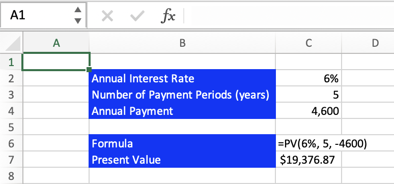
To illustrate the usage of the PV function, let's consider an example. Suppose you want to calculate the present value of an annuity to be paid off over 5 years, with an annual interest rate of 6%, and the payments of $4,600 are made at the end of each year. Below is an image showing the setup and calculation of this example.

It should be pointed out that the optional fv and type arguments have been omitted from the function above. This is because in this situation we are paying at the end of each year and plan on paying the whole thing off. These are the default settings and so while you can input 0 for both these arguments it is not necessary. Additionally, we have the annual payment (pmt) input with a negative sign because it is a deposit.
And so, in this example, the annuity would be worth $19,376.87 today.
Go to the page LiveFlow‘s How to Guides to find more information about Excel and Google Sheets formulas and tips that were not covered here.

