IRR function in Excel: Explained

In this article, you will learn how to use the IRR formula in Excel.

‍

What does the IRR Formula in Excel do?

The IRR function in Excel (Internal Rate of Return) is used to calculate the rate of return at which the net present value (NPV) of a series of cash flows equals zero. In other words, it is the rate of return that makes the present value of all cash inflows equal to the present value of all cash outflows.

The IRR function is often used in financial analysis to evaluate the profitability of an investment or project. A higher IRR indicates a more profitable investment, while a lower IRR indicates a less profitable investment.

‍

How to use the IRR function in Excel?

The syntax of the IRR function in Excel is:

<pre><code>=IRR(values, [guess])</code></pre>

where "values" is the range of cash flows for which you want to calculate the IRR, and "guess" (optional) is your estimate of the IRR. If you omit the "guess" argument, Excel will use a default value of 0.1 (10%).

‍

Case study to demonstrate the use of IRR formula in Excel

Here's a simple case study to demonstrate the use of the IRR function in Excel:

‍

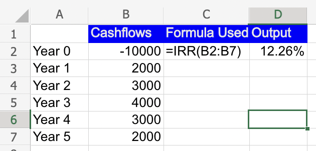
Suppose you are considering investing in a project that requires an initial investment of $10,000 and is expected to generate the following cash flows over the next 5 years:

‍

Year 1: $2,000

Year 2: $3,000

Year 3: $4,000

Year 4: $3,000

Year 5: $2,000

‍

To determine whether this project is worth investing in, you can use the IRR function in Excel as follows:

Step 1: Create a new spreadsheet in Excel and enter the cash flows for each year in a column, starting from cell B2. In this example, you would enter the values in cells B2 through B7.

Step 2: Start with entering the Initial Investment  in Year 0 with negative sign and then the yearly cash flows in Year 1 to 5 with positive sign

Step 3: In the next cell (e.g., cell C2), use the IRR function to calculate the internal rate of return for the project. The formula for cell C2 would be "=IRR(B2:D7)". Note that the range of values passed to the IRR function should include the initial investment (cell B2).

Step 4: Press Enter to calculate the IRR. In this example, the IRR would be 12.26%.

‍

Interpret the result. Since the IRR is higher than the required rate of return (which may be set by the investor or the company), the project is considered to be profitable and may be worth investing in.

‍

Note: Values must contain at least one positive value and one negative value to calculate the internal rate of return.