Custom Number Formatting in Excel
In this article, you will learn what custom number formatting is in Excel and how to apply it.
What is custom number formatting in Excel?
Custom number formatting in Excel is a feature that allows you to change the appearance of date in a cell without altering the actual data. Essentially, this functionality manipulates the visual representation of numbers, dates, times, and text, making it easier to read and interpret. To create a custom number format, you need to understand 2 key elements: sections and the format codes.
Custom number formatting sections
In a custom number format, you can define up to four sections separated by semicolons, each serving a specific purpose.
- The first section formats positive numbers and zeros
- The second formats negative numbers
- The third formats zero values
- The fourth formats text
Below is a visual guideline for these sections.
Note: If you have no formatting for a particular section remember to still include semicolons for empty sections.
Understanding Common Custom Number Format Codes
Format Codes are characters that you type into the custom format box to indicate how numbers should appear. Here are the most commonly used format codes and their explanations:
- 0 (Zero): This is a digit placeholder that displays insignificant zeros if a number has fewer digits than there are zeros in the format, essentially it ensures a minimum number of digits. For instance, 0000 will display the number 5 as 0005. This feature is useful in maintaining uniformity of data, like maintaining a certain length for identification numbers.
- #: This is also a digit placeholder that does not display extra zeros when the number has fewer digits than there are # symbols in the format. So, #### will display 5 as 5.
- . (Period): It is used to represent the decimal point in a number.
- , (Comma): This serves two purposes. Firstly, it can be used as a thousand separator. Secondly, if it follows the digit placeholders (0 or #), it scales the number by a thousand.
- %: It multiplies the number by 100 and displays the number as a percentage.
- E+: It is used to display numbers in scientific notation.
- _ (underscore): It is used to insert a space in a number format that is equal to the width of the character that follows it.
- * (asterisk): It is used to fill the cell with repeated characters.
- @: This symbol is used in the text section of a format to specify where to draw the text in a cell.
- [Color]: This specifies the color for a section. The colors that can be used include Black, Blue, Cyan, Green, Magenta, Red, White, and Yellow.
- General: This displays the number as is, changing only when there are more than 11 digits, at which point it switches to scientific notation.
- Date and Time Codes: There are various codes to display date and time that you can mix together. Below in the next section is a list of these codes and examples.
Custom Formatting Dates and Time
Date and Times have various codes to display date and time.
Day codes: “d” for day, “dd” for day with a leading zero, “ddd” for abbreviated day name, and “dddd” for full day name.
Month codes: "m" for month, "mm" for month with a leading zero, "mmm" for abbreviated month name, and "mmmm" for full month name
Year codes: "y" for year, "yy" for two-digit year, and "yyyy" for four-digit year
Hour codes: "h" for hour and "hh" for hour with a leading zero
Minute codes: "m" for minute and "mm" for minute with a leading zero
Second codes: "s" for second and "ss" for second with a leading zero
Period of day code: "AM/PM" for period of the day
By putting these codes together you can create a custom date and time format. Below are a few examples.
- mm/dd/yyyy: This format will display the date in a month/day/year format. For example, if the date is August 3, 2023, it will appear as 08/03/2023.
- dddd, mmmm dd, yyyy: This will display the date in a full weekday name, month name, day, and year format. For the same date, it will appear as Thursday, August 03, 2023.
- h:mm AM/PM: This will display time with hours and minutes in AM/PM format. For example, if the time is 15:30, it will appear as 3:30 PM.
How to apply and use custom number formatting in Excel
To apply a custom format, select the cells, then right-click and choose Format Cells. In the Number tab, select Custom and type your format into the Type box. Below are a few examples of custom formatting and their results.
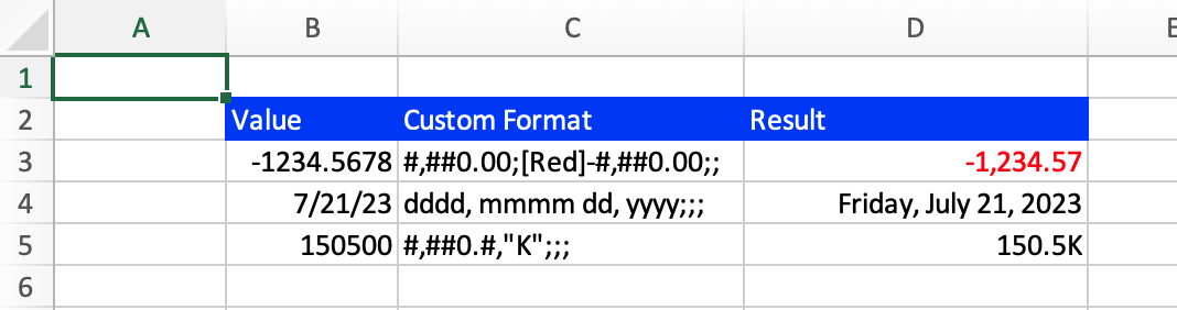
Lets break down one of these custom formats, consider the 1st example. In this example we have the format #,##0.00;[Red]-#,##0.00. This instructs Excel to:
- Use a comma as a thousand separator (represented by #,##0.00 in both the 1st and 2nd section of the custom format).
- Show two decimal places (represented by .00 in the 1st and 2nd section in the custom format).
- Show negative numbers in red and preceded by a minus sign (represented by [Red]-#,##0.00 in the 2nd section).
Now lets consider a custom format that utilizes all 4 sections.
- The first section "$"#,##0.00 formats positive numbers as currency with two decimal places. For example, the number 1234.56 will display as $1,234.56.
- The second section [Red]"$"-#,##0.00 formats negative numbers in red, shows them as currency, and uses a minus sign. So, -1234.56 will display as a red $-1,234.56.
- The third section simply displays the word "Zero" for any cell with a value of 0
- The fourth section "Text: "@ prefixes any text with "Text: ". For instance, if you type Hello into the cell, it will display as Text: Hello.
By leveraging all sections of custom formatting, you can ensure that your data is displayed consistently and intuitively, no matter its nature.
Excel's custom number formatting feature provides powerful tools to improve data readability and interpretation, giving you the freedom to define your own number formats to better fit your specific requirements. While it may take a bit of practice to master, the benefits of clarity and professionalism in your spreadsheets are significant. It's a tool that proves the saying "It's not just what you say, but how you say it" holds true even in data representation.
Go to the page LiveFlow‘s How to Guides to find more information about Excel and Google Sheets formulas and tips that were not covered here.

