How to Highlight Duplicates in Excel (Quick-start Guide)

In this article, you will learn how to highlight and identify duplicate values using the ‘Conditional Formatting’ feature in Excel.

‍

Benefits of highlighting duplicate values in Excel

Highlighting duplicates in Excel workbooks offers several benefits, including:

Data Accuracy and Cleanliness: By identifying duplicates in your Excel sheet, you can eliminate errors and ensure that your data is accurate. Furthermore, highlighting duplicate values helps you keep your data clean and organized, which is essential for efficient data analysis.

Better Data Visualization: Highlighting duplicates in Excel makes it easier to spot patterns and trends in your data. For example: it can be used to quickly identify repeat customers. This can help you gain a deeper understanding of your data and make more informed decisions.

Time-Saving: Manually checking for duplicates can be a time-consuming task, especially if you have a large amount of data in Excel spreadsheets. Highlighting duplicates in Excel automates this process and saves you time.

Improved Data Management: By identifying duplicates, you can make better decisions about how to manage your data. For example, you can decide to delete duplicates or merge them into a single record.

In conclusion, highlighting duplicate values in Excel is a valuable tool for data analysis and management. By automating the process of identifying duplicates, it saves you time and helps you keep your data organized, accurate, and clean.

‍

Using ‘Conditional Formatting’ to highlight duplicates in Excel

Excel provides a simple way to highlight duplicates in a range of cells with its ‘Conditional Formatting’ function. This section will guide you through the process of highlighting duplicates in Excel.

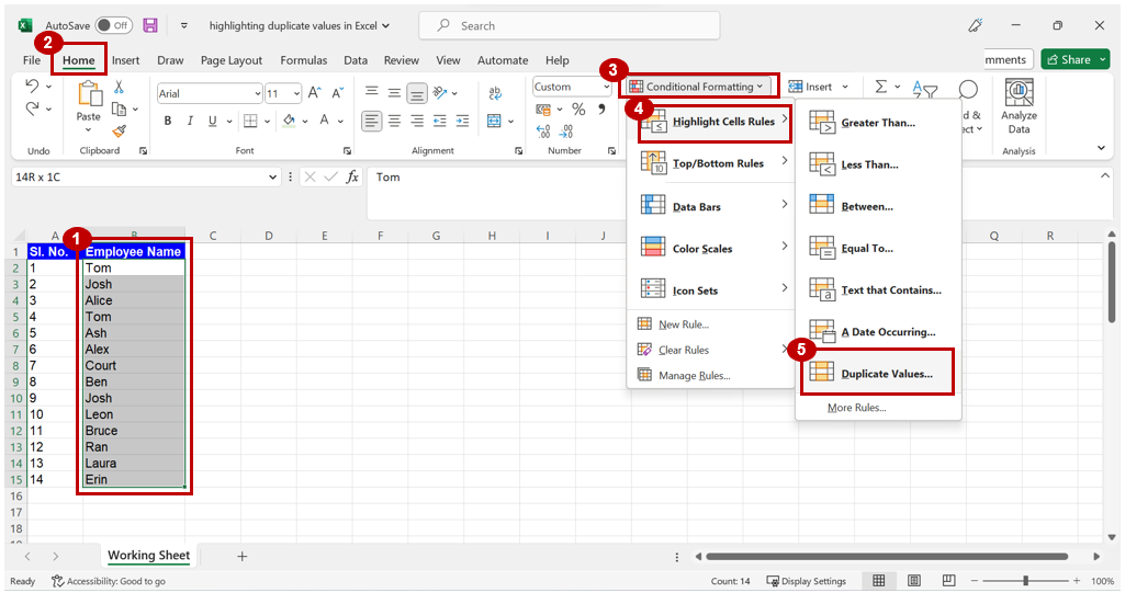
Step 1: Select the range of cells that you want to check for duplicates

Learn how to quickly select adjacent and non-adjacent cells, multiple rows and multiple columns in Excel here:

How to Select Multiple Cells in Excel (Beginner's Guide)

How to Select Multiple Rows in Excel

How to Select Multiple Columns in Excel

‍Step 2: Once you have selected the range of cells, go to the ‘Home’ tab in the Excel Toolbar and click on the ‘Conditional Formatting’ option. From the drop-down menu, select the ‘Highlight Cells Rules’ option and then click on ‘Duplicate Values’.

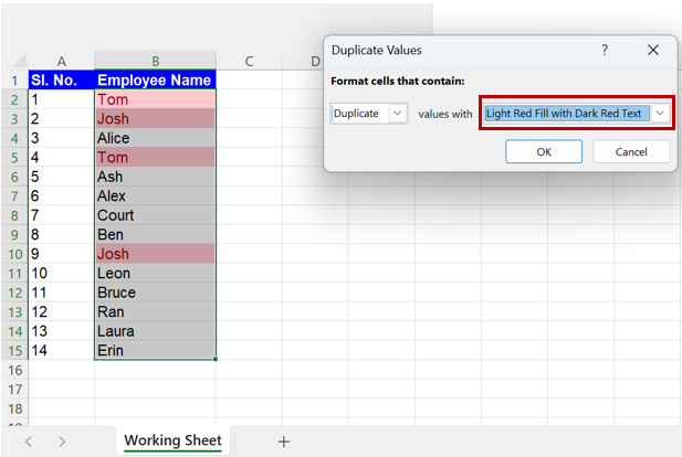
‍Step 3: Excel will show you a dialog box with options to custom format the duplicate values highlighted. You can choose a predefined format from the drop-down list or create a custom format by selecting the ‘Custom Format’ option from the drop-down menu shown in the image below.

‍Step 4: Once you have customized or selected the formatting, click on the ‘OK’ button. Excel will now highlight all the duplicate values in the selected range with the color you specified.

‍

How to remove conditional formatting in Excel

Step 1: Select the range of cells that you want to remove the conditional formatting from

Step 2: Simply go back to the ‘Conditional Formatting’ option and select the ‘Clear Rules’ option. From the drop-down menu, choose ‘Clear Rules from Selected Cells’. The highlights will be cleared from the selected cells. You can also select ‘Clear Rules from Entire Sheet’ to clear conditional formatting from the entire Excel spreadsheet.

‍

And that's a wrap! We hope this article helps you in your data analysis in Excel.

Analyze your live financial data in a snap in Google Sheets

Are you learning this formula to visualize financial data, build a financial model, or conduct financial analysis? In that case, LiveFlow may help you automate manual workflows, update numbers in real-time, and save time. You can access various financial templates on our website, from the simple Income Statement to Multi-Currency Consolidated Financial Statement. Are you interested in this product but are an Excel user? That’s not a problem at all. You can connect Google Sheets to Excel quickly. 

To learn more about LiveFlow, book a demo.

You can learn about other Excel and Google Sheets formulas and tips that are not mentioned here on this page: LiveFlow‘s How to Guides