Applying Conditional Formatting with Formulas in Excel
Excel's conditional formatting feature is incredibly powerful, allowing you to modify the format of cells based on their values. However, many users are unaware that you can increase its functionality by combining it with formulas. This article will explore the use of formulas in Excel's conditional formatting.
What is conditional formatting with formulas in Excel?
Normally, Excel’s conditional formatting uses simple criteria that you specify to determine how to format cells. For instance, you could use a basic rule to highlight cells that are greater than a certain value. However, this can be limiting when you need to apply a rule based on more complex criteria. This is where conditional formatting with formulas comes into the picture. Essentially, it allows you to use a formula to determine the cells in which the formatting is applied. This is a powerful tool because of the versatility of Excel formulas and their ability to handle complex conditions and criteria.
Benefits of conditional formatting with formulas in Excel
Here are a few benefits of using formulas with conditional formatting:
- Versatility: You can use any Excel formula to define your conditions, allowing you to handle more complex scenarios.
- Efficiency: It enables you to automate the process of highlighting important data points, saving you time.
- Clarity: It allows you to make your data visually easier to understand, which can be useful for data analysis and presentation.
How to apply conditional formatting with formulas in Excel
The steps below will guide you on how to apply conditional formatting using formulas:
- Select the range of cells: Click and drag to select the range of cells to which you want to apply conditional formatting.
- Open the conditional formatting menu: Navigate to the Home tab, and in the Styles group click on Conditional Formatting.
- Create a new rule: In the dropdown menu, select New Rule.
- Select rule type: In the New Formatting Rule dialog box, make sure your Style is set to “Classic” and in the next drop down choose “Use a formula to determine which cells to format”.
- Enter your formula: In the box below “Use a formula to determine which cells to format”, input the formula you want to use (Note: The formulas should be written as if you were writing it for the top-left cell for your selected range).
- Specify formatting: Click on the Format with drop down menu to specify the formatting to apply to if conditions of your formula are met. This can involve changing the cell’s fill color, font color, border, etc. Click “OK” when done.
- Apply the rule: Click “OK” again in the New Formatting Rule dialog box to apply the rule. The cells that meet the condition specified by your formula will now have the formatting applied.
Examples of using formulas in conditional formatting in Excel
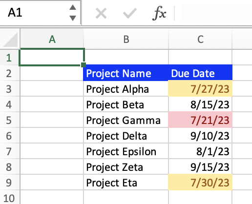
Let's say you're managing a set of projects, and you have an Excel spreadsheet with a column listing the due dates for each project. You can use conditional formatting with formulas to visually indicate how many days are left until each deadline, highlighting tasks that are due soon or already overdue. Below is an image of a data set for this example.
And so, following the steps from earlier, input the wanted formulas. For instance, the deadlines start in cell C3, if you want to highlight tasks due within the next 7 days, the formula would be =AND(C3-TODAY()>=0, C3-TODAY()<=7). This formula checks if the task is due in the next week but is not already overdue. In the Format will specify the format to apply if the formula returns TRUE. In this case we will change the cells fill color and font color to be yellow. Repeat the process to create another rule for overdue tasks. Use the formula =C3<TODAY() and choose a different format, such as a red fill and font color. Below is an image of this example and the conditional formatting with formulas applied.

Now, your spreadsheet will visually indicate tasks that are due soon or already overdue, helping you manage your project more effectively. This is just one situation of many in which you can use conditional formatting with formulas.
Remember, conditional formatting with formula can be as simple or as complex as you need it to be. Your formula can reference multiple cells, use nested functions, or include logical operators. The key is to understand your data and your objectives clearly, so you can construct the formula to suit your needs.
Whether you're working with large datasets or small ones, understanding how to use conditional formatting with formulas can save you time and provide a much richer view of your data. As with many aspects of Excel, practice is key, so start exploring the potential of this feature with your own datasets today.
Go to the page LiveFlow‘s How to Guides to find more information about Excel and Google Sheets formulas and tips that were not covered here.

