Conditional Formatting in Excel: Explained
In this article, you will learn how to use essential functions of Conditional Formatting in Excel.
What is Conditional Formatting in Excel?
Conditional Formatting is a feature in Excel that allows you to apply specific formatting to cells or ranges of cells based on certain conditions. These conditions can be based on cell values, formulas, or other criteria. Conditional Formatting is a powerful tool that can help you quickly identify trends and outliers in your data, and make your spreadsheets more visually appealing and easier to understand.
What are some uses of Conditional Formatting in Excel?
Conditional Formatting is a powerful feature in Microsoft Excel that allows users to apply formatting to cells based on certain conditions or criteria. Some of the common uses of Conditional Formatting in Excel are:
- Highlighting cells that meet certain criteria: For example, you can use Conditional Formatting to highlight all the cells in a column that contain values above or below a certain threshold.
- Color coding data: Conditional Formatting allows you to apply different background colors or font colors to cells based on the values they contain. This makes it easier to identify trends or patterns in your data.
- Creating data bars: Data bars are a visual representation of the values in a range of cells. You can use Conditional Formatting to create data bars that show the relative size of each value in the range.
- Adding icons: Conditional Formatting enables you to add icons to cells based on their values. For example, you can add a green checkmark to cells that meet certain criteria, and a red X to cells that don't.
- Creating heat maps: Heat maps are a visual representation of data that uses color to show the relative values of each cell in a range. You can use Conditional Formatting to create heat maps that make it easy to see patterns in your data.
Overall, Conditional Formatting is a useful tool for analyzing and presenting data in Excel, and can help users to identify trends, patterns, and outliers in their data.
How to use Conditional Formatting in Excel
Here are the steps to use Conditional Formatting in Excel:
Step 1: Select the cells or range of cells that you want to apply Conditional Formatting to.
Step 2: Click on the "Conditional Formatting" button in the "Home" tab of the Excel ribbon.
Step 3: From the dropdown menu, select the type of formatting you want to apply, such as "Highlight Cells Rules" or "Data Bars".
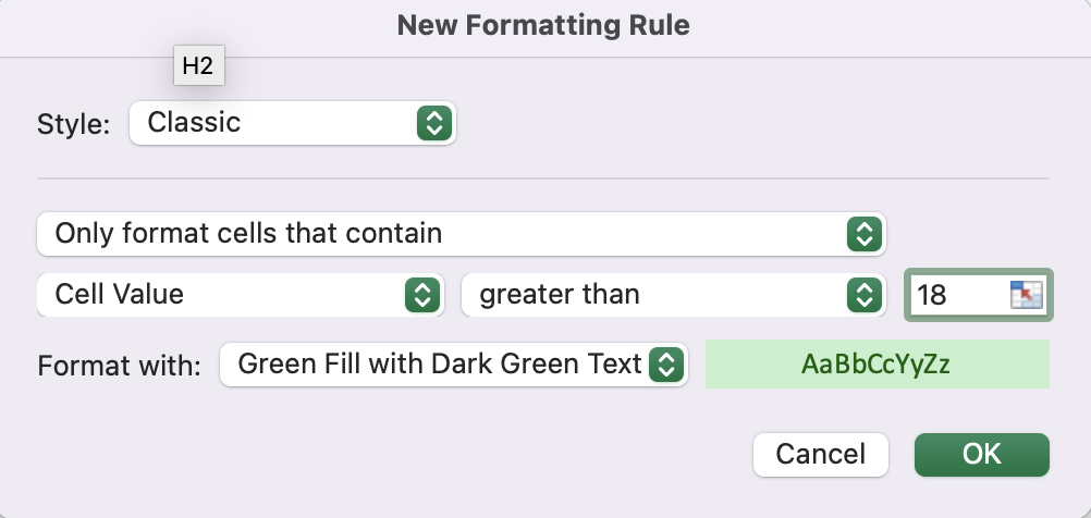
Step 4: Select the specific rule or type of formatting that you want to apply, such as "Greater Than" or "Green Fill with Dark Green Text".
Step 5: Enter the criteria for the formatting rule in the dialog box that appears. For example, if you selected "Greater Than", you would enter the threshold value for the cells that you want to highlight.
Step 6: Customize the formatting options as desired, such as selecting a different color or icon to apply.
Step 7: Click "OK" to apply the formatting rule to the selected cells.


You can also create custom formatting rules in Excel by selecting "New Rule" from the "Conditional Formatting" dropdown menu and entering your own criteria and formatting options. Once you have applied conditional formatting to your Excel worksheet, you can easily modify or remove the formatting by selecting the cells and changing the formatting options in the "Conditional Formatting" dropdown menu.

How to use Conditional Formatting with a practical example
Suppose you are manager for a sales team and wish to track the number of units sold by each of your team members. An easy way to highlight those who sold less than 35 units is to use Conditional Formatting. The spreadsheet has the units sold by employees in column C.
Step 1: Select the range of cells that contain the scores (column C in this case).
Step 2: Click on the "Conditional Formatting" option in the "Home" tab of the Excel ribbon.
Step 3: Select "New Rule" from the dropdown menu. In the "New Formatting Rule" dialog box, select "Highlight Cell Rules" and “Less than...”
Step 4: In the "Cell Value less than" field, enter 35
Step 5: Click on the "Format" button and choose the formatting options that you want to apply to the cells that meet the condition.
Step 6: Click "OK" to close the dialog box.
Now, the cells that contain units sold less than 35 will be highlighted with the formatting options that you chose. As a manager you can quickly see which team members have not met their target.

How to remove Conditional Formatting from cells
Step 1: Put your cursor on a cell or a range that contains a conditional formatting rule you want to remove.
Step 2: Navigate to “Home” and go to “Conditional Formatting”.
Step 3: You have a list of rules applied to the cell.
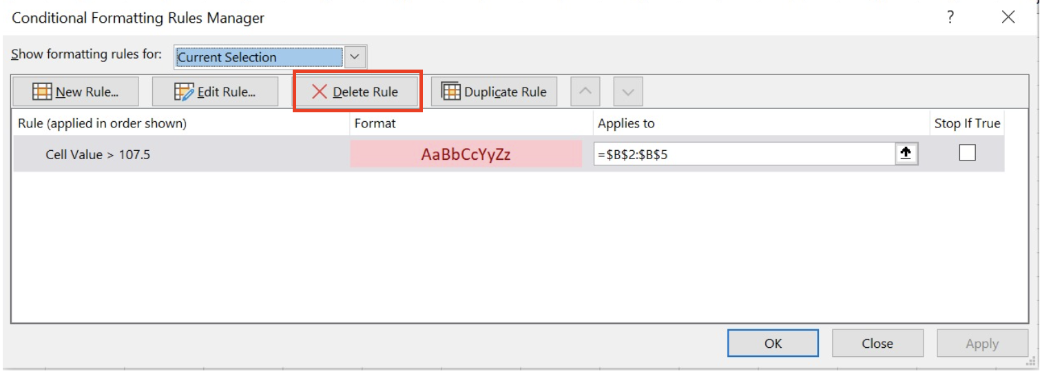
Step 4: Click the “-” sign icon on MAC or “Delete rule” in windows, which pops up when you put your cursor around.


Note: If you want to remove a conditional formatting from a part of the range defined, we recommend you change the selected field in each rule as it allows the rule to be applied to the rest of the area.

