PRODUCT Function in Google Sheets: Explained
In this article, you will learn how to use the PRODUCT formula in Google Sheets.
What is the PRODUCT formula in Google Sheets?
The PRODUCT formula in Google Sheets multiplies all the numbers given as arguments and returns the product.
The PRODUCT function can be beneficial when you have a large number of values to multiply, as it allows you to quickly calculate the product without having to multiply each value manually.
How do you use the PRODUCT function in Google Sheets
To use the PRODUCT function in Google Sheets, follow these steps:
- Select the cell where you want to output the result of the PRODUCT function.
- Type “=PRODUCT”.
- Then type the range of cells you want to multiply, separated by commas. You can also type individual cell references or numbers instead of a range.
- Press the “Enter” key.
Here is the syntax for the PRODUCT formula:
The PRODUCT formula can take multiple arguments, separated by commas. All the arguments must be numeric values.
factor1: A number or a range to be multiplied
factor2: Additional value to be multiplied by
Notes: each factor could be a numeric value or a range containing numbers. If a range, empty cells are ignored in the calculation.
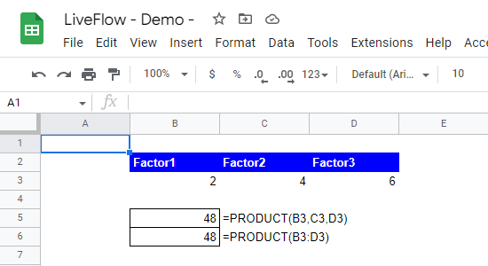
For example, if you have the numbers 2, 4, and 6 in cells B3, C3, and D3, respectively, you can use the PRODUCT formula as follows:
This formula will return result 48, which is the product of 2, 4, and 6.
Here is another example of how you might use the PRODUCT function in Google Sheets:
This formula will multiply the numbers in cells B3, C3, and D3, and return the result in the cell where you entered the formula.
The following picture shows the two examples above.

How to use the SUMPRODUCT formula in Google Sheets
In Google Sheets, you have a similar formula called SUMPRODUCT. The formula multiplies the corresponding entries in a given set of arrays or ranges, and returns the sum of those products.
You can learn about the SUMPRODUCT function here: How to Use SUMPRODUCT Formula in Google Sheets

