How to Use ISERROR in Google Sheets
How to Use ISERROR in Google Sheets
In this article, you will learn how to use the ISERROR function in Google Sheets
What is the ISERROR Function?
The ISERROR function itself is fairly simple: it checks to see if a cell or calculation returns an error. If there is an error, this function will return a value of TRUE, and if there is no error, it will return a value of FALSE. This can be a useful and powerful formula when combined with other functions such as VLOOKUP, IF, SUMIF, or many others.
This creates a multitude of uses for the ISERROR function. Some examples of uses are given below.
Data Validation: When setting up data validation rules, you might want to ensure that the input values don't result in errors. ISERROR can be part of a validation rule to check for potential issues.
Cleaning Data: If you are cleaning and manipulating data, you might encounter errors in the process. ISERROR can help you identify and address these errors.
Conditional Formatting: You can use ISERROR in conjunction with conditional formatting to visually highlight cells that contain errors. This makes it easier to spot and address issues in your data.
VLOOKUP and HLOOKUP: When using VLOOKUP or HLOOKUP functions to search for a value in a table, errors may occur if the lookup value is not found. ISERROR can be used to display any desired text rather than showing an error. Common examples include a blank cell or ‘not found’.
How to Use ISERROR in Google Sheets
ISERROR is a fairly simple function to perform with only one required input. The syntax of ISERROR is as follows:
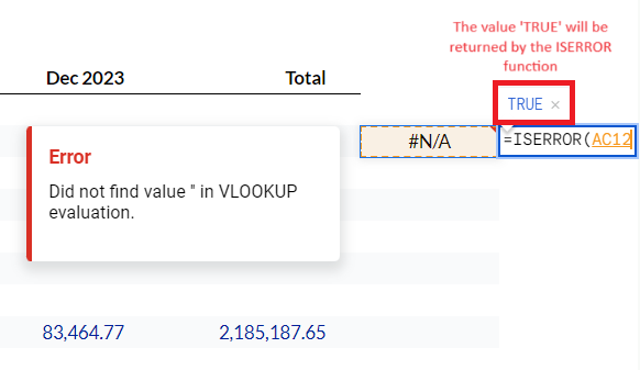
To run the function, just select the value or function you wish to check for an error and Google Sheets will return TRUE or FALSE depending on the error status.
The formula in use should look something like the example below.


