How to Freeze Rows and Columns in Google Sheets
In this article, you will learn how to freeze rows and columns in Google Sheets.
The “Freeze” function is beneficial when you need to handle a vertically and/or horizontally long list in Google Sheets, as you can leave important information (e.g., table headers, names of each item in a table) on your screen while you scroll up, down, right and left.
How to freeze panes in Google Sheets
How to freeze a row
- Select a cell that is a part of the row X up to which you want to freeze.
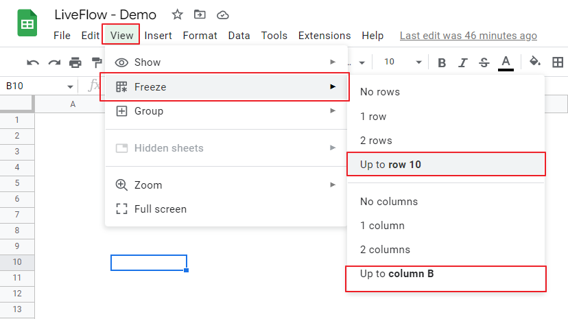
- Go to the “View” tab in the menu bar, ➝ ”Freeze” ➝ ”up to row X”.
- A thick light grey border shows up between row X and row X+1.
- Now rows from Row 1 to X are fixed and stay on your screen; however you scroll.
How to freeze a column
- Select a cell that is a part of the column Y up to which you want to freeze.
- Go to the “View” tab in the menu bar, ➝ ”Freeze” ➝ ”up to column Y”.
- A thick light grey border shows up between column Y and row Y+1.
- Now columns from Column 1 to Y are fixed and stay on your screen; however you scroll.
If you want to freeze both rows and columns, you can combine the two processes above. First you select the cell YX, lock the row or column, and freeze the rest of them.

How to unfreeze panes in Google Sheets
You can unlock rows and columns in almost the same way as you lock them.
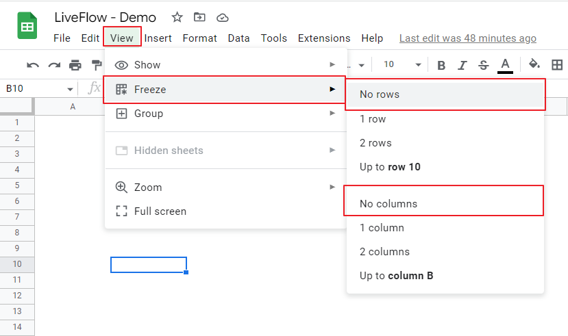
- Go to the “View” tab in the menu bar, and then “Freeze”.
- Choose “No rows” and/or “No columns”.


