UNIQUE Function in Google Sheets: Explained

In this article, you will learn how to use the UNIQUE formula in Google Sheets. The UNIQUE formula is one of the ways to remove duplicates from your data set or pick up different keywords from a list of keywords.

‍

How to use the UNIQUE function in Google Sheets

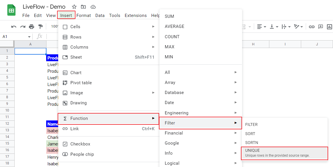
1. Type “=UNIQUE(” or go to “Insert” → “Function” (or directly navigate to the “Functions” icon)  → “Filter” → “UNIQUE”.
2. Select a range from which you delete duplicates.
3. Determine the way of filtering (i.e., by row(s) or column(s) and whether you include the items considered duplicates in the original data) if needed.
4. Press the “Enter” key.

‍

The general formula is as follows:

=UNIQUE(range, [by_column], [exactly_once])

Range: This argument requires a range or an array you want to filter.

By_column (Optional): This parameter defines how the function checks the “range”. You input “FALSE” or “TURE” or keep this item blank. With “FALSE”, the function checks items by rows, and with “TRUE”, it sorts the things by columns. Without any input, the default setting is “FALSE”.

Exactly_once (Optional): This argument determines how the function shows the result. You input “FALSE” or “TURE” or keep this argument blank. With “FALSE”, the function shows things considered duplicates in the original data set (not all of them but one from each duplicate), and with “TRUE”, they are excluded from the result. Without any input, the default setting is “FALSE”.

‍

Notes

1. Secure enough space for the formula to spread its result.
2. Ensure you don’t have the extra space(s) or other hidden texts in each cell in the range to be filtered.
3. Ensure that the items to be sorted have the same formatting (e.g., currency mark).

‍

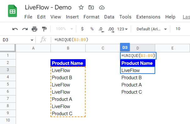
Look at the following example. This picture shows a simple case. In this case, both arguments are blank; thus, the show formula is equivalent to =UNIQUE(B3:B9, “FALSE”, “FALSE”). If you change the “by_column” argument to “TRUE”, the formula shows the same list of items as the range (B3:B9) is considered one item. When you keep the “by_column” parameter blank and input “TRUE” in the last argument, the “exactly_once”, you get a similar sorted list as shown in the screenshot below but without “LiveFlow”, as it is a duplicate in the original list and thus excluded from the result by the parameter.

‍

Finally, see how the formula works for an array. In the following screenshot, the upper table is the initial data set, and the lower table is the result returned by the UNIQUE formula. The highlighted rows are duplicates. Can you see that there is no duplicate in the filtered table? For the “by_column” argument, this example describes how it works better. With “FALSE” input, the formula works by rows, meaning it goes through items grouped like [Isabella/North/20/Plan A] from the top to the bottom, and finds the same items.

‍

How do I prevent duplicates in Google Sheets?

As alternative ways of the UNIQUE function, you can use the Pivot table, Google Sheets’ Data clean-up tool (Remove duplicates), etc. to remove duplicates, and Conditional Formatting to identify duplicates in your data.