How to Remove Duplicates in Google Sheets
There are several ways to get rid of duplicates in Google Sheets: Google Sheets’ “Data cleanup” function, formulas such as the UNIQUE and QUERY, and Pivot Table.
In another way, You can use Conditional Formatting to identify duplicates and remove them manually. In this article, you will learn how to eliminate duplicates using the clean-up function in Google Sheets.
The function is straightforward and valuable when you process the existing data set and don’t need to keep the filtered output dynamic.
How to delete duplicates by Data cleanup in Google Sheets
- Select the range you want to clean up.
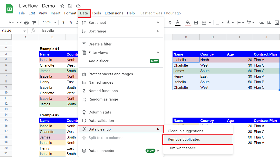
- Go to the “Data” → “Data cleanup” → “Remove duplicates”, which brings up a pop-up menu.
- Check “Data has header now” if the selected range includes table headers.
- Choose the columns based on which duplicates will be removed in the “Columns to analyze” section.
- Click “Romove duplicates”.
Steps 1 and 2

Steps 3 to 5

See the examples below to understand how the function works depending on the number of columns selected in Step 4 above.
Example #1 shows the case in which you select all columns as standard.
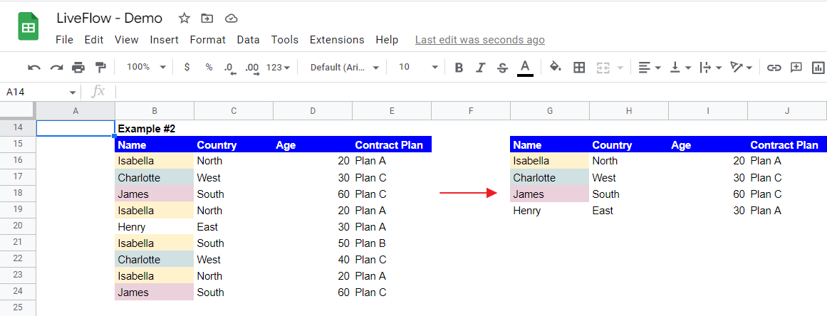
Example #2 presents the outcome when you focus on a single column (Column B - Name)
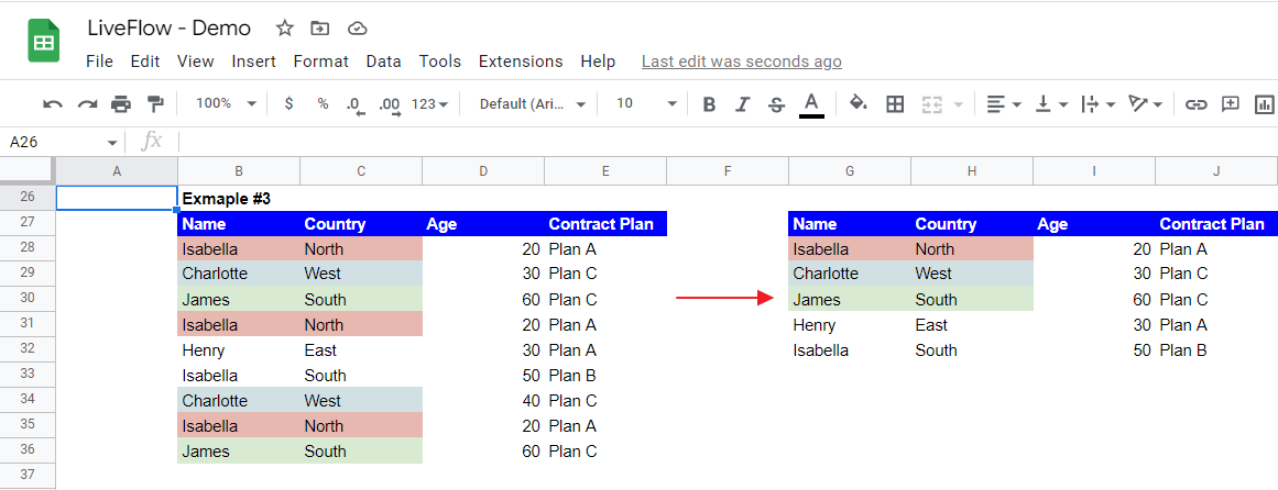
Example #3 describes the case in which you choose two columns for criteria (Column B - Name and Column C - Country)
The entire array, including table headers, is selected as the array to be streamlined and contains the same items in all examples.
Example #1

The highlighted rows are duplicates in the left table. As you can see, after the function is applied, there is no duplication in the table (on the right). The function judges if there is any redundancy based on values in selected columns in a specific row.
For instance, the first row under the headers contains Isabella, North, 20, and Plan A. The function considers the factors as a chunk, and if it finds the same chunk in other rows, it excludes them from the outcome.
Example #2

The function works similarly in this example. However, as we focus on the “Name” column this time, the entire table is rearranged only based on the items in Column B (Name); The rows incorporating identical names are removed.
Example #3

The function works similarly to the first example. In this example, it regards items in Columns B and C in a row as one group and eliminates other rows containing the same information.
Thus, as you can see, even though the sixth row includes the same information (Isabella) for Column B as the first row because their countries are different, the sixth row remains in the streamlined list.
Finally, ensure you don’t have the extra space(s) or other hidden texts in each cell in the range to be filtered.

