HYPERLINK Function in Google Sheets: Explained
In this article, you will learn how to use the HYPERLINK formula in Google Sheets.
What does the HYPERLINK function do in Google Sheets?
The HYPERLINK function in Google Sheets creates a clickable link to a specified URL, file, or email address. It is helpful for creating links within a worksheet that can be clicked to access additional information or to quickly open a file or email without having to leave the worksheet.
For example, you could use the HYPERLINK formula to create a clickable link to a website that contains more information about a particular topic or to a file that contains supporting data for your spreadsheet.
You could also use the formula to create a link to an email address that people can click to send you a message without opening their email program.
How to use the HYPERLINK formula in Google Sheets?
The syntax for the HYPERLINK function is as follows:
URL argument is the URL, file, or email address that you want to create a link to.
Link_label argument is optional and specifies the text displayed as the clickable link. If you do not specify this argument, the link location will be used as the link text.
Note that you need to enclose URL and link_label with quotation marks each when you input them directly in the formula instead of cell references (e.g., HYPERLINK(“https//:liveflow.io”, “LiveFlow”). Otherwise, the formula returns a “#ERROR!” value in a cell.
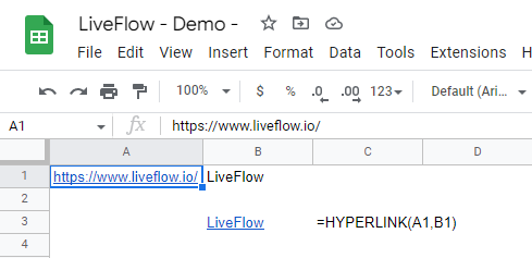
For example, if you have a URL in cell A1 and a text string for a label in cell B1, and want to create a clickable link to that URL in cell B3, you can use the formula =HYPERLINK(A1, B1) in cell B3. This will create a clickable link in cell B3 that will open the URL in cell A1 when clicked.


