Alternate Column Colors in Google Sheets: Explained
In this article, you will learn how to alternate cell colors for every two columns. If you need to learn how to change row color every two rows, check this article: How to Alternate Row Colors in Google Sheets
What is alternating colors in Google Sheets?
Alternating colors means that you change the cell colors for every two rows or columns with two kinds of colors (e.g., white and light grey). It is often applied to a table or list containing a data set to make each row or column clear so that readers can go through the information easily.
How to alternate column color in Google Sheets
Although you can use the Google Sheets tool to alternate row colors, you need to use Conditional Formatting with a custom formula to alternate column colors. It is not difficult but simple as shown below.
- Select the range you want to apply a pattern.
- Navigate to the “Format” tab → “Conditional formatting”.
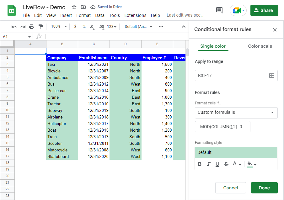
- Choose “Custom formula is” → Enter “=MOD(COLUMN(),2)=0”.
- Click the “Done” button at the bottom right.


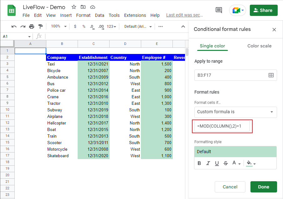
You need to understand that you make the MOD function return 0 (where a column number is even) or 1 (when a column number is odd) by entering 2 as its divider and that the Conditional Formatting you define is applied where the MOD function returns 0. In the example, Conditional Formatting is effective in columns with even numbers. If you want to apply Conditional Formatting to columns with odd numbers, you can change the custom formula to “=MOD(COLUMN(), 2)=1”. You can see the outcome in the picture below.

What does the alternating color function do?
Google sheets’ alternating color function allows you to alternate colors easily but only for rows. You can learn how to use the function in the following articles: How to Alternate Row Colors in Google Sheets

